Tensor-Product Presentation of NTT and Constant-Geometry NTT
Most iterative NTT hardware paper eventually hits the same wall: the butterflies are trivial, and the addressing is where all the design effort goes. Write an NTT as a nest of for loops and you get index expressions like j + (i << (k-l)) scattered across the datapath, changing shape at every stage. The loops are correct but they are not analyzable — you cannot look at them and see which memory access pattern falls out.
Tensor products fix this. They let you write the whole transform as a product of structured matrices, where each factor names one concrete hardware resource: a bank of butterflies, a permutation network, a ROM read. Once the algorithm is an algebraic object, restructuring the dataflow becomes matrix manipulation rather than index bookkeeping.
This note builds that machinery from scratch and then uses it to derive the constant-geometry NTT — the variant where the wiring between stages is literally the same permutation every stage. I follow the derivation in Zhang et al. (FCCM 2023), which presents this in an FHE accelerator context, and I flag at the end where the structure is actually much older than that paper.
Everything below I checked numerically (symbolic DFT over up to , plus integer NTT mod ); the figures are generated from the sparsity patterns of the actual matrices, not drawn by hand.
1. The two patterns that matter
For square matrices and , the tensor (Kronecker) product replaces every entry of with the block , giving a matrix of order .
The entire formalism rests on the fact that two special cases mean two different machines. Let have length .
is block-diagonal with copies of . To see what that demands of memory, you have to say explicitly how is cut into the blocks the copies act on. Partition it into contiguous segments of length :
so segment starts at offset and walks with stride . Under that blocking the product is literally the segments processed one by one:
The index never appears inside the sum. Segment is closed under the operator — PE reads only , writes only , and never talks to its neighbours. That is processors doing the same job on adjacent data, and if you give each PE its own memory bank holding one segment, no two PEs ever address the same bank.
The second pattern is easier to build in the opposite direction: start from the operation you want, and let the matrix fall out of it.
Cut the other way — not segments of length , but subvectors of length :
Now treat each subvector as though it were a single number, and combine the whole set of them using the coefficients of . Output subvector is the weighted sum of all input subvectors, the weights being row of :
There is no matrix product here yet — is just scalar-times-vector products added together, done times over. Note the roles: is the size of the transform, and is how many vectors ride through it together, the width of the machine.
To turn into a single operator on the stacked , use the one observation that does all the work: scaling a length- vector by the scalar is the same as multiplying it by the matrix . So one output block is a row of such matrices applied to ,
and stacking all block rows gives the whole thing:
Now look at what that matrix is. Every entry of has been replaced by the block — which is precisely the tensor product defined at the top of this section, taken with . The operator that forms weighted sums of whole subvectors is the tensor product:
Read by index, says
and the position is untouched — it sits identically on both sides of the sum. Element of every subvector is combined only with element of the others, never with the elements beside it. Collect those matching positions and you get vectors of length ,
one for each . Run that relation backwards and it says the same thing from the other side: subvector collects the -th element of each of the vectors — the first subvector is built from the first element of every , the second from every second element, and so on.
In those terms the whole operation is just , one vector at a time. Concretely at : gather the first element of each of the subvectors, multiply that length- vector by each row of in turn, and the numbers that come out are the first elements of the output subvectors. Then repeat for . So separate -point operations — one per vector, each reading with stride .
That is the whole difference. Both forms are independent copies of ; the only question is which elements one copy sees — offset with stride above, offset with stride here.
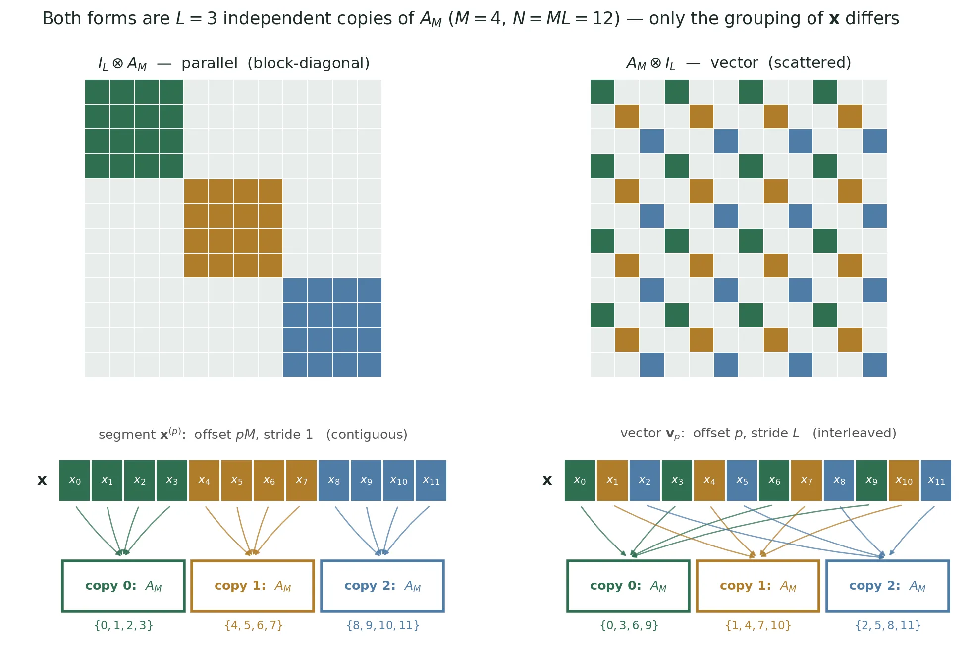
The figure makes the point better than the algebra does. Both panels contain exactly copies of and do exactly the same arithmetic. What changes is the access pattern: contiguous runs on the left, interleaved vectors on the right. Same operator , same data, completely different memory behaviour — and on hardware that difference is a conflict-free bank read versus a strided gather. The whole game is choosing which form you want at each stage.
One more identity we need for scalability. If you have fewer than processors, split the identity:
Read right to left: the inner is a chunk of work, and you hand of those chunks to physical processors. This single line is why the resulting architecture scales to any PE count — more on that in §7.
2. Stride permutation
The data movement operator is the stride permutation , with . Conventions differ between authors, so let me pin mine down explicitly:
In words: read with stride , elements at a time. Output block is . For this is the perfect shuffle — evens then odds:
Three properties carry the derivation.
Factorization. A stride splits into two strides:
Inverse. Taking , and noting :
so strides and undo each other. This is what makes the twiddle matrix stay diagonal in §5.
Commutation theorem. This is the bridge between the two processing styles:
Parallel form and vector form compute the same thing up to a stride permutation. Any algorithm expressed in tensor products can therefore be retargeted — pushed toward parallel or toward vector — by moving permutations around. That is the lever we pull in §4.
3. NTT as a matrix factorization
The NTT of length over maps coefficients by
with a primitive -th root of unity mod (so ). Collecting this into a matrix, with :
It is the DFT with swapped for — same algebra, no rounding error. So every Cooley–Tukey-style factorization transfers verbatim; only the coefficient ring changes.
For the twiddles, define the diagonal matrix
where is a primitive -th root of unity. The general Cooley–Tukey construction stacks powers of down the diagonal, but radix 2 never needs that generality. The only twiddle matrix (5) below ever instantiates is , and , so at every stage and there are always exactly two blocks:
That is just the twiddle structure of a decimation-in-time stage written out: the first half of the coefficients pass through untouched, the second half pick up .
The decimation-in-time factorization into radix-2 butterflies then reads
with the bit-reversal permutation applied to the input. Write for the stage- twiddle matrix.
The product runs left to right, so applied to a vector the stage executes first. Keep this in mind — it is why the figures below run .
A worked example:
Take , so three stages. Everything below stays in terms of alone — a primitive -th root of unity mod — so none of it depends on which you pick.
At stage we have , , and the order- root is . Writing out (6) and (7) stage by stage:
| runs | ||||||
|---|---|---|---|---|---|---|
| 3 | 1st | 1 | 2 | |||
| 2 | 2nd | 2 | 4 | |||
| 1 | 3rd | 4 | 8 |
Two things fall straight out. The stage that executes first has , so — no twiddles at all, which is the familiar fact that the opening decimation-in-time stage is pure add/subtract. And the twiddle set doubles every stage until the last one carries the full .
The butterfly operator changes shape just as fast. pairs coefficients at distance :
| operator | pairs | stride | |
|---|---|---|---|
| 3 | 1 | ||
| 2 | 2 | ||
| 1 | 4 |
Bit reversal first puts the input in the order
and because stage carries no twiddles, it is nothing but four 2-point transforms on adjacent pairs:
Stages and then merge those four 2-point transforms into two 4-point ones and finally a single 8-point one, picking up and then along the way. That last column of the second table — stride — is the whole difficulty, and it is what the next section has to get rid of.
Now look at the operator in the middle:
This is neither of our two clean patterns. It is a mixed three-factor product: independent copies of the vector operation . Worse, both exponents move with . At it is one wide vector operation; at it is independent scalar butterflies. A fixed piece of hardware cannot be both.
4. Flattening to pure parallelism
Getting rid of the mixed form is exactly what stride permutations are for. The three-factor identity is
with . The mixed operator becomes a pure parallel operator sandwiched between two permutations. Substituting into (5) with , , :
This is real progress: the compute operator is now the same at every stage — independent radix-2 butterflies, the ideal parallel form.
But the addressing got worse. Each stage now carries two permutations, and both depend on :
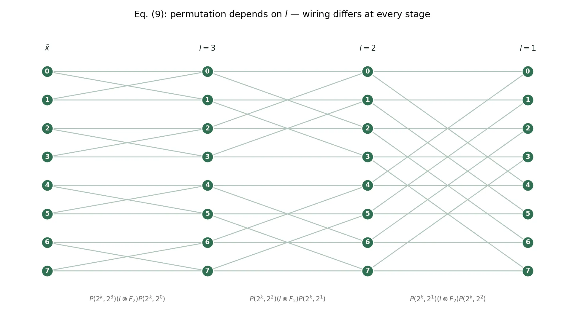
Three stages, three different wiring patterns, two readdressing passes each. In hardware that means either a general-purpose interconnect (expensive, and it degrades badly as and PE count grow) or reconfiguring the address generation per stage. This is the memory-access bottleneck that dominates scalable NTT designs.
5. Deriving constant geometry
Here is the trick. Unfold (9) along and look at the boundaries between adjacent stages:
The leading permutation of stage is . Split it with rule (2):
Only — a plain perfect shuffle, no in it — stays with stage . The leftover is pushed left, out of stage and onto the tail of stage . Do this at every boundary and the shifted factors telescope:
Every stage now has an identical prefix , and the -dependence has been squeezed into the region around the twiddle matrix. Absorb it:
Why is still diagonal. Because , the inverse property from §2 gives . So (13) is a similarity transform of a diagonal matrix by a permutation:
Conjugating a diagonal matrix by a permutation just reorders its diagonal — it can never introduce off-diagonal mass. is diagonal, therefore it moves no data. It is a pure element-wise multiply.
That is the whole point. All stage-dependent data movement has been converted into stage-dependent twiddle-factor selection. Coefficients now flow through the same fixed shuffle every stage; only the ROM addresses change.
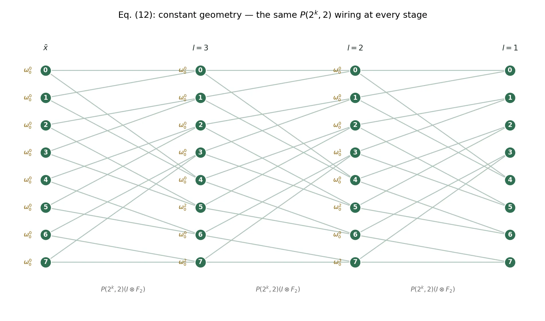
Compare against the previous figure: same butterflies, same number of stages, but one wiring pattern instead of three. This is a constant-geometry algorithm.
The trade is favourable because it is asymmetric: coefficient movement costs you on both the read and the write side every stage, whereas twiddle selection is a read-only lookup in the multiplier stage that never has to relocate anything in memory.
6. Collapsing the twiddle storage
Constant geometry is only a win if the twiddle addressing does not become the new mess. It doesn’t — it collapses to one line of index arithmetic.
Let be the diagonal of . From (6) and (7) it is repetitions of a block:
with primitive of order . By the similarity argument the diagonal of is — segment into groups and deal one element from each group round-robin. The result interleaves into
Two things fall out.
One root for all stages. has order while has order , so
Every stage’s twiddles are powers of the same . No per-stage root tables.
A closed-form address. Every even-indexed coefficient pairs with . For odd index at stage , the required exponent is
Since always, a single table of powers — stored once, in order, never rewritten — serves the entire transform. The exponents in the second figure are computed from (16); I verified it reproduces the exact diagonal of (13) for all stages up to .
So the “hard” part of the memory access pattern reduces to a shift and a mask.
7. What this buys in hardware
Scalable PE count. Split the butterfly bank using identity (1). With PEs and :
Each PE handles butterflies. is now a free parameter — the same algorithm covers a 1-PE area-minimal design and a 64-PE throughput design with no restructuring. Each stage takes cycles, so latency is butterfly slots.
Fixed interconnect. never changes, so read/write addressing is generated once at elaboration time from and . The control unit shrinks to a counter plus (16) — which is what actually makes routing tractable as grows, since a stage-varying permutation network is what usually caps the achievable frequency.
Ping-pong memory. The transform is not in-place under a fixed shuffle, so you need two banks, alternating by the parity of . That is the honest cost of constant geometry: coefficient storage instead of . You are buying wiring simplicity with memory.
The paper’s Algorithm 1, which is (12) written as loops:
k = log2(N);  beta = 2^(k-1) / alpha
x = bit_reverse(x)
for l = k down to 1:
    for i = 0 to alpha-1:          # parallel across PEs
        for j = 0 to beta-1:       # sequential within a PE
            d  = i*beta + j
            w  = w0 ^ ( floor((2*d+1) / 2^l) * 2^(l-1) )    # eq (16)
            v[d]           = x[2*d] + x[2*d+1] * w   mod q
            v[d + 2^(k-1)] = x[2*d] - x[2*d+1] * w   mod q
    x = v
return x
The write pattern d and d + 2^(k-1) is — the shuffle never appears as an explicit permutation step, it is just where the two butterfly outputs get written. I implemented this against a naive NTT mod for and ; all match.
8. Two caveats
This is Pease’s algorithm. Zhang et al. state theirs is “the first work to apply tensor products to NTT designs.” The tensor-product formalism for FFTs is standard and long-established — Tolimieri, An & Lu is the canonical treatment, and it is the paper’s own reference [25]; the SPIRAL project is built on it. More specifically, equation (12) is the Pease FFT (1968), transplanted from to : constant geometry with a fixed stride permutation and bit-reversed input is precisely what Pease derived. That does not diminish the accelerator — applying it to FHE-scale parameters with a scalable PE count and getting good silicon out is real work — but the derivation in §4–§6 is classical FFT theory, and it is worth knowing that so you can read the older literature for the variants.
This is the cyclic NTT, not the negacyclic one. Algorithm 1 advertises but computes the plain length- cyclic transform — I confirmed this by testing against the cyclic definition, which is what it matches. RLWE-based FHE needs negacyclic convolution, which requires folding in powers of with : pre-scale , post-scale by , or use the standard merged- butterflies that absorb the scaling into the twiddle tables. That last option is what real designs do, and it changes the twiddle table contents but not the geometry — so §5 survives intact. Worth stating explicitly, because the omission is easy to miss.
Where I want to take this next: the same manipulation with a different split point gives the four-step / six-step decompositions, which is how you get NTTs whose working set fits in on-chip memory at FHE parameter sizes. Same algebra, different factorization — which is the real argument for the tensor-product view.
References
- Y. Zhang, S. R. Sathi, Z. Kou, S. Sinha, W. Zhang, “Tensor-Product-Based Accelerator for Area-efficient and Scalable Number Theoretic Transform,” FCCM, 2023. DOI: 10.1109/FCCM57271.2023.00027 — the source of the derivation in §3–§7.
- R. Tolimieri, M. An, C. Lu, Algorithms for Discrete Fourier Transform and Convolution, Springer, 1997 — the standard reference for the tensor-product/stride-permutation formalism. §1–§2 here is a compressed version of its opening chapters.
- M. C. Pease, “An Adaptation of the Fast Fourier Transform for Parallel Processing,” JACM 15(2), 1968 — the original constant-geometry FFT.
- C. Van Loan, Computational Frameworks for the Fast Fourier Transform, SIAM, 1992 — the clearest catalogue of FFT variants in Kronecker notation.
- M. Püschel et al., “SPIRAL: Code Generation for DSP Transforms,” Proc. IEEE 93(2), 2005 — tensor-product factorizations as a machine-searchable space.
- A. C. Mert, E. Karabulut, E. Öztürk, E. Savaş, A. Aysu, “An Extensive Study of Flexible Design Methods for the Number Theoretic Transform,” IEEE Trans. Computers, 2020 — the scalable iterative-NTT baseline Zhang et al. compare against.
- A. C. Mert, E. Öztürk, E. Savaş, “Design and Implementation of Encryption/Decryption Architectures for BFV Homomorphic Encryption Scheme,” IEEE TVLSI 28(2), 2020 — the 64-PE iterative and four-step comparison points.
- P. Longa, M. Naehrig, “Speeding up the Number Theoretic Transform for Faster Ideal Lattice-Based Cryptography,” CANS, 2016 — the merged- negacyclic construction referenced in §8.